Technical directors new to waste-to-energy are often surprised to learn calorific value is not a fixed property of "waste" the way it might be treated on paper. It moves through the year, for reasons that have nothing to do with plant performance. Seasonal calorific value variation is a known feature of municipal solid waste streams, driven by what households and businesses discard differently in different months. A permit condition or combustion control setpoint written around a single annual average can look wrong for weeks at a time, even when nothing at the plant has changed.
This is not a minor operational curiosity. It shapes how permit reporting should be framed, how combustion planning should account for the calendar, and how a compliance manager tells a genuine seasonal pattern apart from an emerging operational problem.
The mechanism: moisture content and organic fraction drive the seasonal swing
The underlying driver is straightforward. Calorific value is inversely related to moisture content, and strongly influenced by the proportion of the waste stream that is plastics versus biodegradable organic material. When moisture rises or the organic fraction expands relative to plastics, calorific value falls; when the reverse happens, it rises.
A 2025 study in Nature Scientific Reports examined the physio-chemical properties of municipal solid waste across dry and wet seasons and found the plastics fraction shifting from 21.45% in the dry season to 26.94% in the wet season, with the biodegradable fraction holding around 35% in both. That study was conducted in Uganda, and the specific percentages are not representative of European waste streams; collection systems, climate, packaging mix, and organics collection differ substantially. What transfers is the mechanism, not the numbers: moisture content and the plastics-to-organics balance are the physical drivers of seasonal calorific value change, wherever the waste originates. In Europe, the same mechanism plays out through different seasonal patterns, holiday waste, garden waste volumes, heating-season packaging, producing a real but differently-shaped swing than the one in that paper.
No reliable published figure exists for a typical European seasonal calorific value swing at plant level, and this article will not manufacture one. What can be stated with confidence is the direction of the mechanism, and that it is real, measurable, and worth planning around.
What this means for permit conditions written around an annual average
Under the 17. BImSchV framework governing incineration and co-incineration of waste in Germany, and its equivalents elsewhere, permit conditions and reporting obligations are frequently anchored to average calorific value and combustion parameters over a reporting period. An annual average is a reasonable regulatory instrument, but it can obscure the fact that the plant spent parts of the year meaningfully above or below that average, not because of a fault, but because of what was in the delivery stream that month.
This matters in two directions. A plant tuned to an outdated seasonal assumption can drift out of its optimal band unnoticed until a stack emissions report flags it. And when a regulator asks why a month's figures deviate from the annual average, "seasonal composition change" is only credible if backed by delivery-level data, not asserted after the fact.
Distinguishing seasonal drift from a real operational problem
The practical difficulty: seasonal calorific value drift and a genuine operational problem, a contaminated delivery stream, a carrier misrepresenting composition, a shift in a supplying region, can look similar from the combustion control room. Both show up as calorific value moving away from where it normally sits. The response differs completely: one calls for adjusted combustion planning, the other for intervention at the gate or with a specific carrier.
How continuous per-delivery measurement tells the two apart
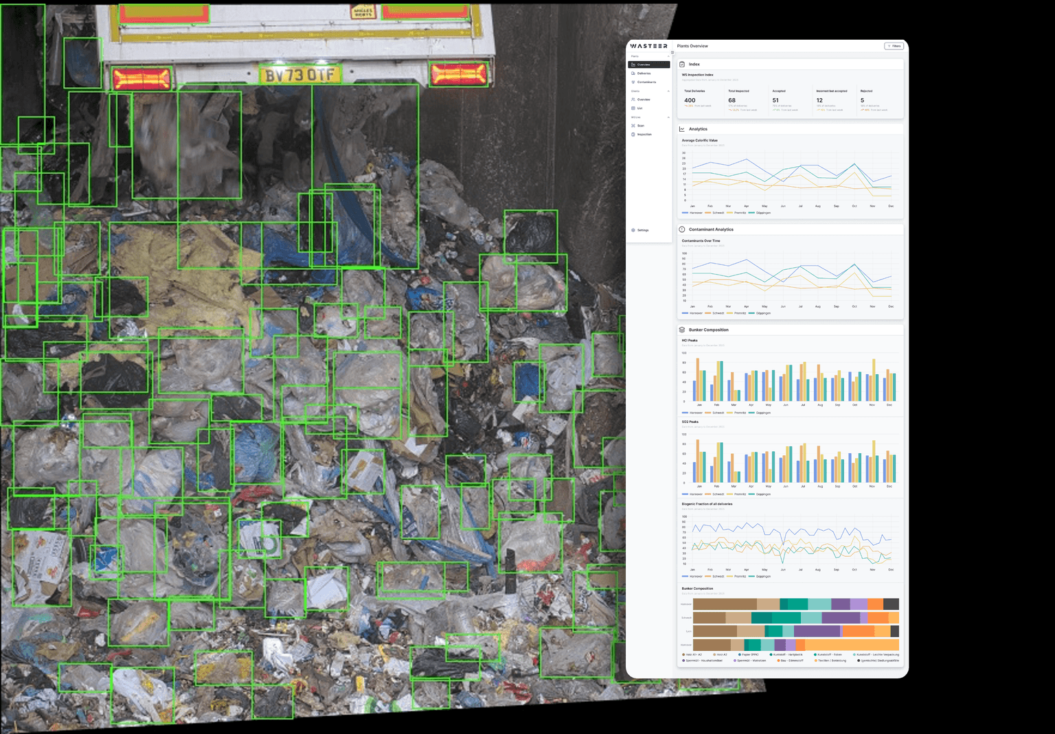
The distinction is visible at the delivery level long before it is visible at the boiler. A seasonal shift is gradual and broad-based across many deliveries and carriers over weeks. A genuine problem is a sharp deviation concentrated in specific deliveries or carriers, against a seasonal baseline that otherwise holds steady. This is only distinguishable with continuous per-delivery measurement rather than periodic sampling; a monthly composite sample cannot tell a plant whether a low-calorific-value week reflects the whole intake shifting or three unusual loads landing in the same sampling window. Wasteer's camera-based system covers how per-delivery calorific value estimates are generated continuously, making this pattern-versus-anomaly read possible, rather than reconstructed after the fact from boiler behaviour.
Building seasonal variation into reporting and combustion planning rather than treating every swing as an anomaly
Once a plant has a season-by-season view of its own delivery stream, the practical response is to build that pattern into planning rather than treat it as a yearly surprise: combustion control expectations that anticipate the calendar, permit reporting deviations flagged proactively with seasonal context attached, and investigation effort reserved for deviations that don't fit the established pattern. It also lets the plant distinguish, in its reporting narrative, "expected winter pattern" from "needs explanation," a stronger position with a regulator than treating every deviation as equally uncertain.
This connects directly to combustion stability: why a stable calorific value band matters at the boiler applies whether the band shifts from a real anomaly or a seasonal pattern. Either way, the plant benefits from knowing which one it is looking at before adjusting support firing or grate settings.
What the aggregate install base shows about variability reduction regardless of season
Reporting from EUWID Recycling in December 2025 on Wasteer's install base across 28 facilities in 7 countries found calorific value standard deviation reduced by 10 to 15% on average, and 40 to 60% for extreme outlier deliveries, alongside throughput increases of 2 to 8% and reductions in operating resource consumption of 8 to 17%. These figures describe the aggregate pattern across the install base; they are not a guarantee for any individual facility, and no single named customer's results are represented.
It is worth being precise about what this means. Continuous per-delivery measurement does not remove seasonal variation in the underlying waste stream, and does not "solve seasonality." It makes swings visible and manageable sooner, whether the cause is a seasonal shift in moisture and organic fraction or an operational issue at the gate. That earlier visibility produces the standard deviation reduction: not a smoother waste stream, but a plant reacting faster, with better information about what kind of variability it is facing.
FAQ
Does calorific value really change enough between seasons to matter, and can we cite that in a regulatory audit? The mechanism is well established. Magnitude at any individual European plant depends on local collection patterns and climate; there is no published EU-wide figure to cite. "Waste changes seasonally" alone is unpersuasive in an audit. What makes it credible is delivery-level data showing the pattern at your own facility, distinct from anomalous events.
How is seasonal drift different from a contaminant or composition problem we should be investigating? Seasonal drift is broad-based and gradual across many deliveries and carriers. An operational problem concentrates in specific deliveries or carriers, breaking from the seasonal baseline. Distinguishing the two requires continuous, per-delivery data rather than periodic composite sampling.
Should combustion control setpoints change by season? That is a plant-specific decision, but it should be informed by the plant's own seasonal delivery data, not a generic assumption. A plant with a documented seasonal pattern can plan support firing, grate settings, and reporting expectations around the calendar, rather than treating every month as identical to the annual average.
For a broader view of how continuous composition data supports compliance reporting generally, see why stable, continuous composition data matters for compliance reporting.